
Until recently, VoLCA used MUMPS for its matrix computations. MUMPS is a well-established sparse direct solver written in Fortran and used far beyond LCA. Replacing it was not an obvious choice.
My curiosity came mainly from two questions. Could Rust make the computations much faster than MUMPS? And what might a Haskell implementation achieve? The new Fable 5.2 made it possible to explore both approaches quickly.
I assigned the two approaches to two Fable 5.2 agents and told each of them, “Let’s see who wins.” One wrote the solver in Rust with an FFI bridge to Haskell. The other stayed directly in the engine’s language.
I expected Rust to win by a factor of at least two. The surprise was how well the Haskell solver performed: almost level with the Rust solver on routine queries, and well ahead on the large batch measured on my laptop.
Why change a solver that worked?
In VoLCA, calculating a product inventory means solving a system of the form:
(I − A)x = dA represents exchanges between processes, d the final demand, and x the activity levels needed to meet it.
MUMPS solved the vast majority of these systems correctly and quickly. But its integration had costs beyond the time spent on the computation itself.
The build had to combine Haskell, C, Fortran, MUMPS, and OpenBLAS on Linux, macOS, and Windows. On Windows, several dynamic libraries had to accompany the executable. Within the engine, the solver’s native state required locks and a queue: two requests using the same database could not solve their systems at the same time.[1]
Another problem was less visible. When two processes each consumed all of the other’s output, the system had no useful answer. With our MUMPS integration and its settings, the computation could still return finite numbers. They looked like a normal result, but had no meaningful interpretation.[1]
The initial goal was therefore fairly modest: simplify the build, remove the locks, and explicitly reject systems with no solution.
Two approaches, Rust and Haskell
The first approach used Rust. It included a Cargo workspace, a sparse solver, an FFI interface with Haskell, and all the integration required across the five build platforms. This stack was taken through testing, then retained in several branches and pull requests as a reference.[2]
The second agent wrote another implementation directly in Haskell.
Both approaches used the particular structure of a technosphere matrix, but they were not organized in exactly the same way. The Haskell version works loop by loop, chooses an elimination order that limits matrix fill-in, then stores the factors as immutable data. The Rust approach included a dense tail and an FFI bridge. In both cases, several requests could read the same factors concurrently.[1][2]
This is not a general replacement for every sparse solver. It uses the properties of the LCA problem handled by VoLCA.
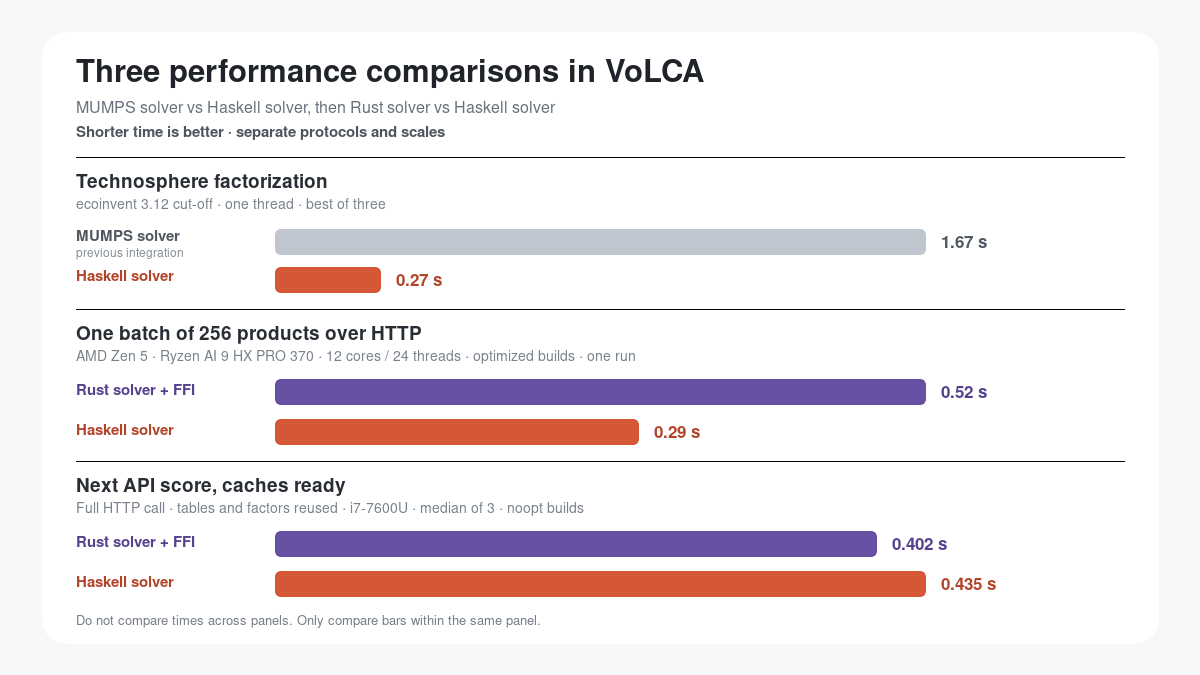
On my laptop, with a 12-core/24-thread AMD Zen 5 processor, the two solvers had almost identical throughput for supply chains and scores. Haskell processed a batch of 256 products in 0.29 seconds, compared with 0.52 for Rust, and a supply chain after a change in 0.58 seconds, compared with 0.66. On the machine hosting this work, an API call with warm caches takes 0.402 seconds with Rust and 0.435 with Haskell. That machine uses an Intel Core i7-7600U, with two cores and four hardware threads. Intel dates its launch to the third quarter of 2016.[6] The protocols differ, so I do not infer a general rule about processors from them. The useful observation is simpler: Haskell was at the same level as Rust, far from the twofold gap I had expected.
The Haskell version was ultimately selected, and the Rust stack was closed the same day.[1][2]
The artifacts from both approaches remain available in their CI runs.[4][5]
The Haskell approach also had a smaller source code footprint. Its three modules contained 1,243 lines. The Rust approach contained 2,019 lines in its crates, or 2,208 including the Haskell bridge needed to call it. The two implementations were not divided up in exactly the same way. This raw count, which includes comments and blank lines, measures neither code quality, difficulty, nor complexity.
The Haskell Linux binary from CI is 18,757,560 bytes, compared with 19,181,196 bytes for the Rust approach, about 2.2% smaller.[4][5] This compares those two builds, not a complete before-and-after comparison with MUMPS. The broader change is that MUMPS, OpenBLAS, the Fortran runtime, and their bindings are gone. On Windows, the archive now contains only one executable and its license files.[1]
The three measurements that surprised me
The three comparisons do not follow exactly the same protocol. I keep them separate rather than constructing a single ranking.
1. Haskell versus MUMPS
The pull request reports the following internal measurements on a technosphere of 26,500 processes, using one thread. The hardware, number of repetitions, and exact definition of peak memory are not documented there. These figures should therefore be read as the result of this experiment, not as a general and directly reproducible benchmark. The MUMPS figure of 1.8 ms is its best case, in batch processing.[1]
| Operation | MUMPS | Haskell solver |
|---|---|---|
| Factorization | 1.67 s | 0.27 s |
| One solve | 1.8 ms | 0.5 ms |
| Peak memory | 403 MB | 101 MB |
With six threads, 2,400 solves take 4.58 seconds with the old integration and 0.54 seconds with the new one.[1]
Part of the gap under concurrency comes from the architecture, not only from the numerical computation. Our MUMPS integration sat behind global locks. The Haskell factors are immutable: each request creates its own workspace and solves in parallel.
Factorization itself is still faster in this measurement. The new solver has neither an optimized dense kernel nor special vector instructions. On this technosphere, a specialized method and a suitable elimination order mattered more than calling a general-purpose numerical library.
2. Almost level on a 12-core AMD Zen 5, with Haskell ahead on batches
The protocol was preserved in perf/solver-choice.md. It compared three engines over HTTP, one at a time, using ecoinvent 3.12 cut-off and EF 3.1. The Rust and Haskell versions were compiled at optimization level 1. The machine used an AMD Zen 5 processor, Ryzen AI 9 HX PRO 370, 12 cores/24 threads. This was a single run per engine on that machine.
| Measurement through the engine | Rust | Haskell |
|---|---|---|
| Supply chains per second, 1 / 6 / 24 concurrent requests | 6.8 / 15.1 / 21.6 | 6.8 / 14.9 / 22.1 |
| Scores per second, 1 / 6 / 24 concurrent requests | 7.0 / 16.9 / 22.6 | 6.7 / 16.7 / 22.2 |
| One batch of 256 products | 0.52 s | 0.29 s |
| Four batches of 64 sent together | 0.35 s | 0.32 s |
| Supply chain after a change, median of 60 | 0.66 s | 0.58 s |
| Score with supplier replacement, median of 30 | 0.16 s | 0.16 s |
Routine queries are therefore neck and neck. Haskell is well ahead on the batch of 256 products, slightly ahead on four parallel batches and on recomputation after a change, and level on supplier replacement. Above all, this is far from the general twofold advantage I expected Rust to have.
3. Rust slightly ahead on a warm call with an Intel Core i7-7600U
We then used the two Linux CI artifacts on an Intel Core i7-7600U, launched in the third quarter of 2016, with two cores and four hardware threads.[6] The test calls the API end to end on the BAFU 2026 v1 corpus, using noopt CI builds. It therefore measures more than the solver alone. Each value below is the median of three runs, alternating the order of the two binaries.[4][5]
score_activities call for one activity | Rust | Haskell |
|---|---|---|
| Score started immediately after loading | 21.04 s | 25.39 s |
| Next score, after preparation with factors reused | 0.402 s | 0.435 s |
The timer covers the complete score_activities HTTP call and stops after the response has been decoded. Database loading, however, starts method preparation in the background. Both measured artifacts predate the fix that prevents a score arriving too early from repeating this preparation.[7] The first call starts immediately after loading. If it arrives before the background work has finished, its time may include or be affected by preparation of factor-flow mappings and characterization tables, factorization, solving, inventory and score calculation, then serialization, local HTTP transport, and JSON decoding.
The supplementary measurement retained with the benchmark gives the scale from another run on this 12-core AMD Zen 5 processor: preparing the 320,000 factors in EF 3.1 takes about 8 seconds. Once that preparation is complete, the first score takes 0.5 seconds, including 0.3 for matrix factorization. Before the fix, a score arriving during preparation could repeat that work and slow down factorization.[7]
The 21.04 and 25.39 second figures are therefore not solver benchmarks, and I no longer use them in the chart. The next call is easier to interpret: with the tables and factors reused, the complete Rust request takes about 8% less time. This remains an API measurement on noopt builds, not an isolated measurement of the solve. The difference from the measurements on the 12-core AMD Zen 5 should not be explained by the processor alone: the corpora, compiler options, and measured operations differ.
All of ecoinvent 3.13 in about 2 minutes on an old dual-core i7
I then wanted to measure a complete calculation with the current Haskell engine, rather than an old noopt CI artifact. I compiled commit 4d47df6f with -O2 and GHC 9.12.4, then loaded ecoinvent 3.13 cut-off and EF 3.1 on the same dual-core Intel Core i7-7600U.[8]
Before starting the timer, I let the engine load the database from its cache, list the activities, prepare the method, and perform an initial factorization. The measurement then covers 110 sequential score_activities calls in batches of 250 activities. It includes the engine computation, serialization, local HTTP transport, and JSON decoding. It excludes database extraction, parsing, and loading, as well as the initial preparation and factorization.
Each of the three complete runs took a little over 2 minutes. Every run produced all 25 EF 3.1 scores for all 27,400 processes: 685,000 scores, with no missing, invalid, unscorable, or unsolvable activity.
This is not the time required to import ecoinvent. It is the scoring time after loading and preparation, with local HTTP and JSON still included.
The numerical result was even more interesting
The difference between the two solvers did not exceed 3 × 10⁻¹¹ on any of the measured matrices except one. On that matrix, it reached 1.5 × 10⁻⁸.
We therefore had to determine which result was closer to the solution. An extended-precision refinement gave an unexpected answer: the new solver was within 10⁻¹⁴ of the reference, compared with 1.5 × 10⁻⁸ for the old one.[1]
This does not prove that a small Haskell solver is generally more accurate than MUMPS. It only shows that, on this matrix and with our integration and settings, the divergence did not come from the new code.
The change also improves the handling of matrices with no answer. An impossible loop is no longer turned into plausible numbers. The engine preserves it as an explicit rejection and names one of the processes involved. In a batch calculation, activities that can be calculated are returned normally, while those that reach the loop are listed separately.[3]
The solver retains an important limitation: it does not swap rows. A regular matrix whose diagonal pivot became zero could therefore be rejected as though it had no solution. None of the matrices measured during this experiment triggered that case.[1]
Epilogue: Haskell in the age of AI?
Haskell does not always reassure development teams. Its reputation as a difficult language is real. The developer pool is smaller, some libraries are less familiar, and the learning curve can deter new contributors.
This experiment does not measure the effect of AI or show that Haskell is the best language for agents. It only reinforces a personal hypothesis: typing, immutability, and precise compiler feedback may make assisted code production and review easier.
AI does not remove the maintenance risk. A project still needs people who can understand its choices, review changes, and take responsibility for a release.
But assistance tools may change the cost of learning a demanding language. The type system closes off some wrong directions before execution. Immutable values limit some concurrency errors. The compiler provides quick feedback before the numerical and domain tests even begin.
I see the same benefits in the user interface with Elm, which VoLCA also uses: explicit types, immutable data, and a compiler that reports inconsistencies precisely. This experiment does not measure the effect of AI on Elm development either. It simply suggests that the same constraints can help an agent produce a change that is easier to review.
Haskell requires careful formulation. That formulation can become a useful specification when code is produced with assistance. The compiler does not guarantee that the algorithm is correct, but it narrows the space of acceptable programs. In this rewrite, the selected approach also avoided an additional FFI layer.
What I take from this
I do not conclude that numerical libraries should be rewritten in Haskell, or that a specialized solver will always beat a general-purpose one.
The conclusion is narrower: when a problem has a strong structure, representing it directly may be worthwhile instead of paying the cost of a more general abstraction. That requires comparing answers, looking for systems with no solution, measuring time and memory, and keeping an independent reference for numerical discrepancies.
That verification turned a risky experiment into an acceptable change. The most surprising result is not only that the new computation is faster on the measured technosphere. An approach with a smaller source code footprint, written in the language already used by the engine, also exposed cases where our old integration accepted answers it never should have.
Sources
[1] https://github.com/ccomb/volca/pull/827 [2] https://github.com/ccomb/volca/pull/826 [3] https://github.com/ccomb/volca/pull/832 [4] https://github.com/ccomb/volca/actions/runs/42963355061 [5] https://github.com/ccomb/volca/actions/runs/43066687145 [6] https://www.intel.com/content/www/us/en/products/sku/97466/intel-core-i77600u-processor-4m-cache-up-to-3-90-ghz/specifications.html [7] https://github.com/ccomb/volca/pull/837 [8] https://github.com/ccomb/volca/commit/4d47df6f1111e1fac4bedd6102e0f294fe17bf5f